A Pythonic data science project: Part III
[1]
Part III: Model development
To follow the following article without any trouble, I would recommend to start with the beginning.
How does predictive modeling work
Keep the terminology in mind
This is important to understand the principles and sub-disciplines of machine learning. We are trying to predict a specific output, our information of interest, which is the category of bank note we observe (genuine or forged). This task is therefore labeled as supervised learning, as opposed to unsupervised learning which consists of finding patterns or groups from data without a priori identification of those groups.
Supervised learning can further be labeled as classification or regression, depending on the nature of the outcome, respectively categorical or numerical. It is essential to know because the two disciplines don’t involve the same models. Some models work in both cases but their expected behavior and performance would be different. In our case, the outcome is categorical with two levels.
How does classification work?
Based on a subset of the data, we train a model, so we tune it to minimize its error on these data. To make a parallel with Object-Oriented Programming, the model is an instance of the class which defines how it works. The attributes would be its parameters and it would always have two methods (functions usable only from the object):
- train the model from a set of observations (composed of predictive variables and of the outcome)
- predict the outcome given some new observations Another optional method would be adapt which takes new training data and adjusts/corrects the parameters. A brute-force way to perform this is to call the train method on both the old and new data, but for some models a more efficient technique exists.
Independent evaluation
A last significant element: we mentioned using only a subset of the data to train the model. The reason is that the performance of the model has to be evaluated, but if we compute the error on the training data, the result will be biased because the model was precisely trained to minimize the error on this training set. So the evaluation has to be done on a separated subset of the data, this is called cross validation.
Our model: logistic regression
This model was chosen mostly because it is visually and intuitively easy to understand and simple to implement from scratch. Plus, it covers a central topic in data science, optimization. The underlying reasoning is the following: The logit function of the probability of a level of the classes is linearly dependent on the predictors. This can be written as:
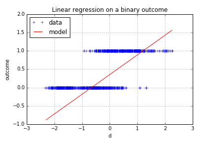
np.log(p/(1-p)) = beta0 + beta[0] * x[0] + beta[1] * x[1] + ...Why do we need the logit function here? Well technically, a linear regression could be fitted with the class as output (encoded as 0/1) and the features as predictive variables. However, for some values of the predictors, the model would yield outputs below 0 or above 1. The logistic function equation yields an output between 0 and 1 and is therefore well suited to model a probability.
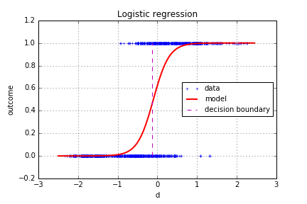
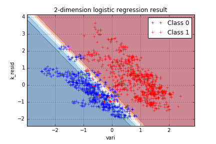
You can noticed a decision boundary, which is the limit between the region where the model yields a prediction “0” and a prediction “1”. The output of the model is a probability of the class “1”, the forged bank notes, so the decision boundary can be put at p=0.5, which would be our “best guess” for the transition between the two regions.
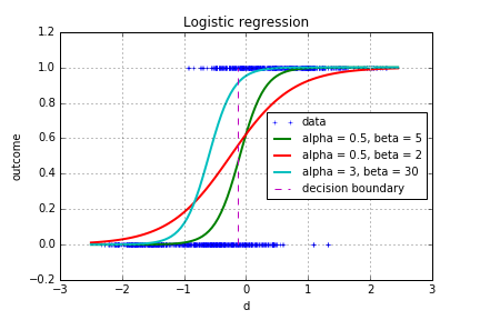
Required parameters
As you noticed in the previous explanation, the model takes a vector of parameters which correspond to the weights of the different variables. The intercept \beta_0 places the location of the point at which p=0.5, it shifts the curve to the right or the left. The coefficients of the variables correspond to the sharpness of the transition.
Learning process
Parameters identification issue
Unlike linear regression, the learning process for logistic regression is not a straight-forward computation of the parameters through simple linear algebra operations. The criterion to optimize is the likelihood, or equivalently, the log-likelihood of the parameters:
L(beta|(X,z)) = f(X,z)Parameters update
The best parameters in the sense of the log-likelihood are therefore found where this function reaches its maximum. For the logistic regression problem, there is only one critical point, which is also the only maximum of the log-likelihood. So the overall process is to start from a random set of parameters and to update it in the direction that increases the log-likelihood the most. This precise direction is given by the gradient of the log-likelihood. The updated weights at each iteration can be written as:
beta = beta + gamma* gradient_log_likelihood(beta)Several criteria can be used to determine if a given set of parameters is an acceptable solution. A solution will be considered acceptable when the difference between two iterations is low enough.
Optimal learning rate
The coefficient gamma is called the learning rate. Higher values lead to quicker variations of the parameters, but also to stability and convergence issues. Too small values on the other increase the number of steps required to reach an acceptable maximum. The best solution is often a varying learning rate, adapting the rate of variations. The rate at step n is chosen as follows:
gamma_n = alpha*min(c0,3/(np.sqrt(n)+1))Which means that the learning rate is constant for all first steps until the following condition is reached:
n > (3-c0)/c0After this iteration, the learning rate slowly decreases because we assume the parameters are getting closer to the right value, which we don’t want to overshoot.
Decision boundaries and 2D-representation
A decision region is the subset of the features space within which the decision taken by the model is identical. A decision boundary is the subset of the space where the decision “switches”. For most algorithms, the decision taken on the boundary is arbitrary. The possible boundary shapes are a key characteristic of machine learning algorithms.
In our case, logistic regression models the logit of the probability, which is strictly monotonous with the probability as linearly proportional to the predictors. It can be deduced that the decision boundary will be a straight line separating the two classes. This can be visualized using two features of the data, “vari” and “k_resid”:
w = learn_weights(data1.iloc[:,(0,1,3)])

# building the mesh
xmesh, ymesh = np.meshgrid(np.arange(data1["vari"].min()-.5,data1["vari"].max()+.5,.01),\
    np.arange(data1["k_resid"].min()-.5,data1["k_resid"].max()+.5,.01))

pmap = pd.DataFrame(np.c_[np.ones((len(xmesh.ravel()),)),xmesh.ravel(),ymesh.ravel()])
p = np.array([])
for line in pmap.values:
    p = np.append(p,(prob_log(line,w)))

p = p.reshape(xmesh.shape)

plt.contourf(xmesh, ymesh, np.power(p,8), cmap= 'RdBu',alpha=.5)
plt.plot(data1[data1["class"]==1]["vari"],data1[data1["class"]==1]["k_resid"],'+',label='Class 0')
plt.plot(data1[data1["class"]==0]["vari"],data1[data1["class"]==0]["k_resid"],'r+',label='Class 1')
plt.legend(loc="upper right")
plt.title('2-dimension logistic regression result')
plt.xlabel('vari')
plt.ylabel('k_resid')
plt.grid()
plt.show()
Implementation
Elementary functions
Modularizing the code increases the readability, we define the implementations of two mathematical functions:
def prob_log(x,w):
    """
    probability of an observation belonging
    to the class "one"
    given the predictors x and weights w
    """
    return np.exp(np.dot(x,w))/(np.exp(np.dot(x,w))+1)
def grad_log_like(X, y, w):
    """
    computes the gradient of the log-likelihood from predictors X,
    output y and weights w
    """
    return np.dot(X.T,y- np.apply_along_axis(lambda x: prob_log(x,w),1,X)).reshape((len(w),))
Learning algorithm
A function computes the optimal weights from iterations to find the maximal log-likelihood of the parameters, using the two previous functions.
def learn_weights(df):
    """
    computes and updates the weights until convergence
    given the features and outcome in a data frame
    """
    X = np.c_[np.ones(len(df)),np.array(df.iloc[:,:df.shape[1]-1])]
    y = np.array(df["class"])
    niter = 0
    error = .0001
    w = np.zeros((df.shape[1],))
    w0 = w+5
    alpha = .3
    while sum(abs(w0-w))>error and niter < 10000:
        niter+=1
        w0 = w
        w = w + alpha*min(.1,(3/(niter**.5+1))) * (grad_log_like(X,y,w))
    if niter==10000:
        print("Maximum iterations reached")
    return w
Prediction
Once the weights have been learnt, new probabilities can be predicted from explanatory variables.
def predict_outcome(df,w):
    """
    takes in a test data set and computed weights
    returns a vector of predicted output, the confusion matrix
    and the number of misclassifications
    """
    confusion_matrix = np.zeros((2,2))
    p = []
    for line in df.values:
        x = np.append(1,line[0:3])
        p.append(prob_log(x,w))
        if (prob_log(x,w)>.5) and line[3]:
            confusion_matrix[1,1]+=1
        elif (prob_log(x,w)<.5) and line[3]:
            confusion_matrix[1,0]+=1
        elif (prob_log(x,w)<.5) and not line[3]:
            confusion_matrix[0,0]+=1
        else:
            confusion_matrix[0,1]+=1
    return p, confusion_matrix, len(df)-sum(np.diag(confusion_matrix))
Cross-validated evaluation
Learning weights on a training subset and getting the error on an other subset will allow us to estimate the real error rate of our prediction. 100 cross validations are performed and for each of them, we add the error to a list.
error = []
weights = []
for test in range(100):
    trainIndex = np.random.rand(len(data0)) < 0.85
    data_train = data1[trainIndex]
    data_test = data1[~trainIndex]
    weights.append(learn_weights(data_train))
    error.append(predict_outcome(data_test,weights[-1])[2])
The following results were obtained:
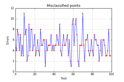
The model produces on average 2.66 mis-classifications for 100 evaluated banknotes. Note that on each test, 85% of the observations went into the training set, which is arbitrary. However, too few training points would yield inaccurate models and higher error rates.
Improvement perspectives and conclusion
On this data set, we managed to build independent and reliable features and model the probability of belonging to the forged banknotes class thanks to a logistic regression model. This appeared to be quite successful from the error estimation on the test set. However, few further progresses could be made.
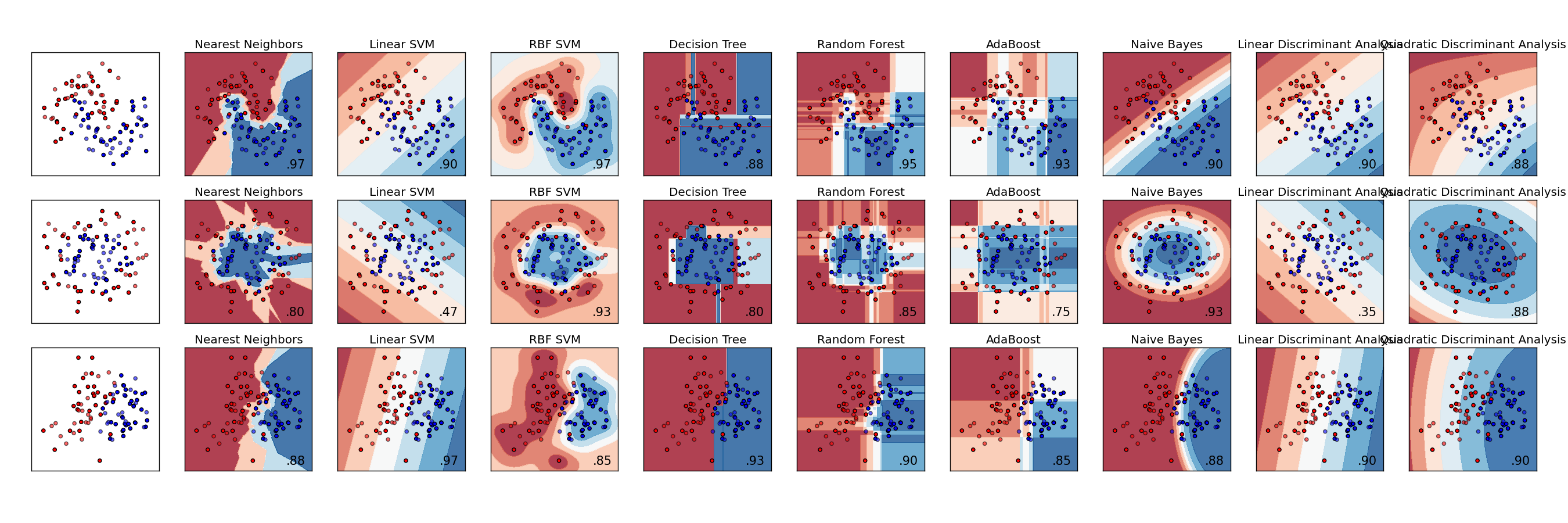
Testing other models
We only implemented the logistic regression from scratch, given that several models would have increased the length of this article. But some other algorithms would have been interesting, such as:
- K nearest neighbors
- Support Vector Machine
- Model-based predictions such as naive Bayes or Quadratic Discriminant Analysis
- Classification Tree
Fact of interest: the two first algorithms also build linear decision boundaries, but based on other criteria.
Adjusting the costs
We assumed that misclassifying a true banknote was just as bad as doing so for a forged one. This is why using a limit at p=0.5 was the optimal choice. But suppose that taking a forged banknote for a genuine one costs twice more than the opposite error. Then the limit probability will be set at p = 0.25 to minimize the overall cost. More generally, a cost matrix can be built to minimize the sum of the element-wise product of the cost matrix with the confusion matrix. Here is an interesting Stack Overflow topic topic on the matter.
Online classification
The analysis carried on in this article is still far from the objective of some data projects, which would be to build a reusable on-line classifier. In our case, this could be used by bank to instantaneously verify bank notes received. This raises some new issues like the update of different parameters and the detection of new patterns.
Special thanks to Rémi for reading the first awful drafts and giving me some valuable feedback.
Mathieu Besançon
Researcher in mathematical optimization
Mathematical optimization, scientific programming and related.