DifferentialEquations.jl came to be a key component of Julia’s scientific ecosystem. After checking the JuliaCon talk of its creator, I couldn’t wait to start building stuff with it, so I created and developed a simple example detailed in this blog post. Starting from a basic ordinary differential equation (ODE), we add noise, making it stochastic, and finally turn it into a discrete version.

Before running the code below, two imports will be used:

import DifferentialEquations
const DiffEq = DifferentialEquations
import Plots

I tend to prefer explicit imports in Julia code, it helps to see from which part each function and type comes. As DifferentialEquations is longuish to write, we use an alias in the rest of the code.

The model

We use a simple 3-element state in a differential equation. Depending on your background, pick the interpretation you prefer:

1. An SIR model, standing for susceptible, infected, and recovered, directly inspired by the talk and by the Gillespie.jl package. We have a total population with healthy people, infected people (after they catch the disease) and recovered (after they heal from the disease).

2. A chemical system with three components, A, B and R. $$A + B → 2B$$ $$B → R$$

After searching my memory for chemical engineering courses and the universal source of knowledge, I could confirm the first reaction is an autocatalysis, while the second is a simple reaction. An autocatalysis means that B molecules turn A molecules into B, without being consumed.

The first example is easier to represent as a discrete problem: finite populations make more sense when talking about people. However, it can be seen as getting closer to a continuous differential equation as the number of people get higher. The second model makes more sense in a continuous version as we are dealing with concentrations of chemical components.

A first continuous model

Following the tutorials from the official package website, we can build our system from:

• A system of differential equations: how does the system behave (dynamically)
• Initial conditions: where does the system start
• A time span: how long do we want to observe the system

The system state can be written as: $$u(t) = \begin{bmatrix} u₁(t) \
u₂(t) \
u₃(t)
\end{bmatrix}^T $$

With the behavior described as: $$ \dot{u}(t) = f(u,t) $$ And the initial conditions $u(0) = u₀$.

In Julia with DifferentialEquations, this becomes:

α = 0.8
β = 3.0
function diffeq(du, u, p, t)
    du[1] = - α * u[1] * u[2]
    du[2] = α * u[1] * u[2] - β * u[2]
    du[3] = β * u[2]
end
u₀ = [49.0;1.0;0.0]
tspan = (0.0, 1.0)

diffeq models the dynamic behavior, u₀ the starting conditions and tspan the time range over which we observe the system evolution. Note that the diffeq function also take a p argument for parameters, in which we could have stored $\alpha$ and $\beta$.

We know that our equation is smooth, so we’ll let DifferentialEquations.jl figure out the solver. The general API of the package is built around two steps:

1. Building a problem/model from behavior and initial conditions
2. Solving the problem using a solver of our choice and providing additional information on how to solve it, yielding a solution.

prob = DiffEq.ODEProblem(diffeq, u₀, tspan)
sol = DiffEq.solve(prob)

One very nice property of solutions produced by the package is that they contain a direct way to produce plots. This is fairly common in Julia to implement methods from other packages, here the ODESolution type implements Plots.plot:

Plots.plot(sol)

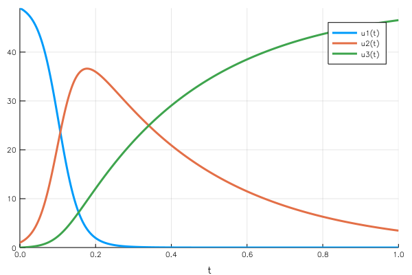
If we use the disease propagation example, $u₁(t)$ is the number of healthy people who haven’t been infected. It starts high, which makes the rate of infection by the diseased population moderate. As the number of sick people increases, the rate of infection increases: there are more and more possible contacts between healthy and sick people.

As the number of sick people increases, the recovery rate also increases, absorbing more sick people. So the “physics” behind the problem makes sense with what we observe on the curve.

A key property to notice is the mass conservation: the sum of the three elements of the vector is constant (the total population in the health case). This makes sense from the point of view of the equations: $$\frac{du₁}{dt} + \frac{du₂}{dt} + \frac{du_3}{dt} = 0$$

Adding randomness: first attempt with a simple SDE

The previous model works successfully, but remains naive. On small populations, the rate of contamination and recovery cannot be so smooth. What if some sick people isolate themselves from others for an hour or so, what there is a meeting organized, with higher chances of contacts? All these plausible events create different scenarios that are more or less likely to happen.

To represent this, the rate of change of the three variables of the system can be considered as composed of a deterministic part and of a random variation. One standard representation for this, as laid out in the package documentation is the following: $$ du = f(u,t) dt + ∑ gᵢ(u,t) dWᵢ $$

In our case, we could consider two points of randomness at the two interactions (one for the transition from healthy to sick, and one from sick to recovered).

Stochastic version

σ1 = 0.07
σ2 = 0.4
noise_func = function(du, u, p, t)
    du[1] = σ1 * u[1] * u[2]
    du[3] = σ2 * u[2]
    du[2] = - du[1]  - du[3]
end

stoch_prob = DiffEq.SDEProblem(diffeq, noise_func, u₀, tspan)
sol_stoch = DiffEq.solve(stoch_prob, DiffEq.SRIW1())

Note that we also change the solver provided to the solve function to adapt to stochastic equations. The last variation is set to the opposite of the sum of the two others to compensate the two other variations (we said we had only one randomness phenomenon per state transition).

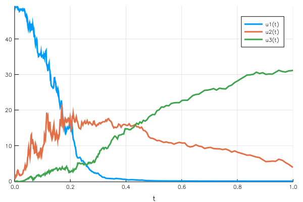
Woops, something went wrong. This time the mass conservation doesn’t hold, we finish with a population below the initial condition. What is wrong is that we don’t define the variation but the gᵢ(u,t) function, which is then multiplied by dWᵢ. Since we used the function signature corresponding to the diagonal noise, there is a random component per $uᵢ$ variable.

Adding randomness: second attempt with non-diagonal noise

As explained above, we need one source of randomness for each transition. This results in a $G(u,t)$ matrix of $3 × 2$. We can then make sure that the the sum of variations for the three variables cancel out to keep a constant total population.

noise_func_cons = function(du, u, p, t)
    du[1, 1] = σ1 * u[1] * u[2]
    du[1, 2] = 0.0
    du[2, 1] = - σ1 * u[1] * u[2]
    du[2, 2] = - σ2 * u[2]
    du[3,1] = 0.0
    du[3,2] = σ2 * u[2]
end
sde_cons = DiffEq.SDEProblem(
    diffeq, noise_func_cons, u₀, tspan,
    noise_rate_prototype=zeros(3,2)
)
cons_solution = DiffEq.solve(sde_cons, DiffEq.EM(), dt=1/500)

We also provide a noise_rate_prototype parameter to the problem builder to indicate we don’t want to use a diagonal noise.

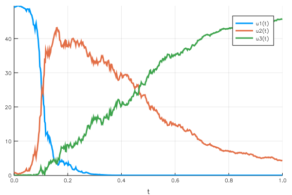
This time the population conservation holds, at any point in time the sum of the $uᵢ(t)$ remains 50.

Discretizing: Gillespie model

The models we produced so far represent well the chemical reaction problem, but a bit less the disease propagation. We are using continuous quantities to represent discrete populations, how do we interpret 0.6 people sick at a time?

One major strength of the package is its effortless integration of discrete phenomena in a model, alone or combined with continuous dynamics. Our model follows exactly the package tutorial on discrete stochastic problems, so building it should be straightforward.

infect_rate = DiffEq.Reaction(α, [1,2],[(1,-1),(2,1)])
recover_rate = DiffEq.Reaction(β, [2],[(2,-1),(3,1)])
disc_prob = DiffEq.GillespieProblem(
    DiffEq.DiscreteProblem(round.(Int,u₀), tspan),
    DiffEq.Direct(),
    infect_rate, recover_rate,
)
disc_sol = DiffEq.solve(disc_prob, DiffEq.Discrete());

We define the infection and recovery rate and the variables $uᵢ$ that are affected, and call the Discrete solver. The Plots.jl integration once again yields a direct representation of the solution over the time span.

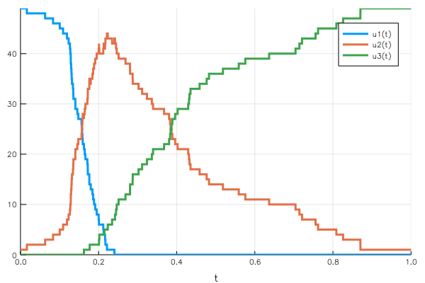
Again, the conservation of the total population is guaranteed by the effect of the jumps deleting one unit from a population to add it to the other.

Conclusion

The DifferentialEquations.jl package went from a good surprise to a key tool in my scientific computing toolbox. It does not require learning another embedded language but makes use of real idiomatic Julia. The interface is clean and working on edge cases does not feel hacky. I’ll be looking forward to using it in my PhD or side-hacks, especially combined to the JuMP.jl package: DifferentialEquations used to build simulations and JuMP to optimize a cost function on top of the created model.

Thanks for reading, get on touch on Twitter for feedback or questions ;)

Edits:

I updated this post to fit the new DifferentialEquations.jl 4.0 syntax. Some changes are breaking the previous API, it can be worth it to check it out in detail.

Chris, the creator and main developer of DifferentialEquations.jl, gave me valuable tips on two points which have been edited in the article. You can find the thread here.

• Import aliases should use const PackageAlias = PackageName for type stability. This allows the compiler to generate efficient code. Some further mentions of type-stability can be found in the official doc
• The second attempts uses non-diagonal noise, the “:additive” hint I passed to the solve function does not hold. Furthermore, the appropriate algorithm in that case is the Euler-Maruyama method.

Many thanks to him for these tips, having such devoted and friendly developers is also what makes an open-source project successful.